Sailing To Philadelphia

Posted on April 9, 2016 by Brian Haren

I am Jeremiah Dixon
I am a Geordie boy
A glass of wine with you, sir
And the ladies I’ll enjoy

All Durham and Northumberland
Is measured up by my own hand
It was my fate from birth
To make my mark upon the earth

He calls me Charlie Mason
A stargazer am I
It seems that I was born
To chart the evening sky

They’d cut me out for a baking bread
But I had other dreams instead
This baker’s boy from the west country
Would join the Royal Society

We are sailing to Philadelphia
A world away from the coaly Tyne
Sailing to Philadelphia
To draw the line
A Mason-Dixon line

It’s amazing where you find historical references. I was listening to a radio talk show the other day and one of the bumper music selections was a duet by Mark Knopfler and James Taylor titled ‘Sailing to Philadelphia‘. The ballad tells the tale of Charles Mason and Jeremiah Dixon, surveyors who, in the mid-1700s, surveyed the boundary between the colonies of Maryland, Pennsylvania and Delaware. The song drew me back to a subject that has fascinated me for a long time – the story of the great boundary survey and how two talented individuals had such a huge impact on scientific and political history.

The Calvert family, which controlled Maryland, and the Penn family, which controlled Pennsylvania and Delaware, had been clashing for years over the boundary between the two colonies. At points the conflict became violent, and as European settlers pushed westward in both colonies the need to firmly establish the boundary became critical. In 1732 the Calverts and Penns agreed on a definition of the boundary: starting at a point formed by the intersection of a line of latitude set 15 miles south of the southernmost limit of the City of Philadelphia and a line of longitude that runs tangent to an 12 mile arc centered on the town of New Castle in Delaware. This definition of a political border as an arc highlights why politicians, particularly politicians with a weak grasp of geometry, should never be allowed to define borders.

After at least one bungled attempt to survey the border it became clear that the task required the best surveyors trained in the newest methods and using the best surveying and time keeping equipment available. In 1761 England’s Royal Astronomer James Bradley recommended two uniquely talented astronomers and surveyors, Charles Mason and Jeremiah Dixon, to tackle the job. Bradley also made sure they were backed by all the resources of the Royal Society and equipped by London’s best instrument makers.

The Royal Society properly viewed the task as one of the greatest scientific and technical challenges of the 18th century, a mission that would have far wider benefit to mankind than just marking a border between to quarreling colonies. It would help prove the utility of longitude determination using chronometers, would test the accuracy and precision of survey instruments made by England’s top makers, would establish the world’s longest and most precise survey baseline and ultimately would return data needed to help establish the precise length of a degree of latitude.

The Mason – Dixon line is actually two lines, or line segments. The east-west line, set at a latitude described as ‘15 miles south of the the southernmost limit of the City of Philadelphia and running five degrees of longitude westward from the Delaware River‘ is what is commonly viewed as the ‘Mason-Dixon line’. However, the north-south segment, set as a line tangent to a 12 mile arc centered in New Castle, Delaware, was actually the most challenging part of the survey. Establishing a line on the ground that is tangent to a continuous arc was a particularly difficult surveying challenge, and one that had never been successfully attempted before Mason and Dixon tackled it

Mason and Dixon had worked together for the Royal Society in the past and were an excellent team. They were also two of the most experienced field surveyors and astronomers of their time. No better team could have been found – their skills, experience, dedication and drive were unmatched.

Mason and Dixon arrived in Philadelphia in late 1763 and set immediately to work. They determined the southern boundary of the City of Philadelphia, established the latitude by astronomical observation, surveyed 31 miles west along the same line of latitude to clear the Delaware River and its local tributaries and established an observatory at a farm owned by John Harland. On Harland’s property they set a monument known as the Stargazers’ Stone on the same line of latitude they had determined at the southernmost boundary of Philadelphia.

The ‘Stargazers’ Stone’ set by Mason & Dixon just north of Harland Farm in Embreeville, Pa.

In 1764 Mason and Dixon ran a survey line 15 miles south of Harlan’s farm and set an oak post (called the Post mark’d West by the surveyors) at 39° 43′ 26.4″ north latitude. This post marked a latitude point precisely 15 miles south of the southernmost limit of the City of Philadelphia. It served as the origin point, or point of beginning, for the survey.

For the remainder of 1764 Mason and Dixon worked on the north – south portion of the line to better define the border between Maryland and Delaware (remember – this was partly defined as a line tangent to a 12 mile arc arc centered on New Castle, Delaware).

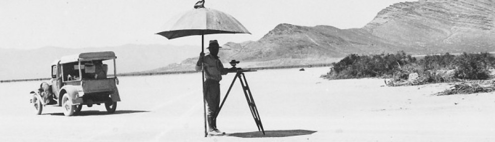
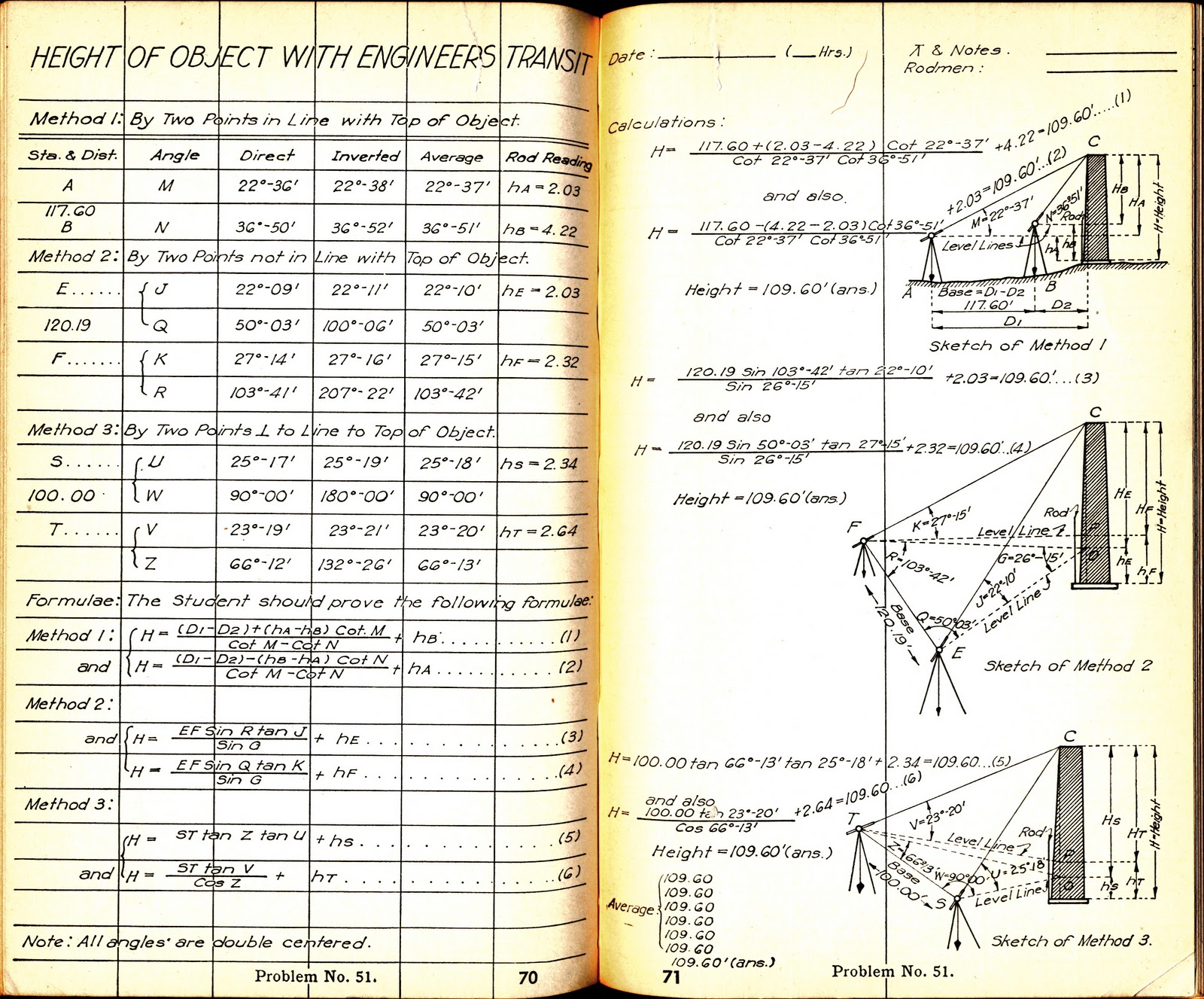
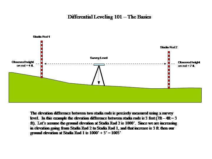
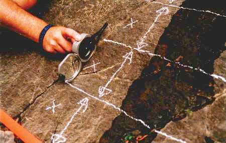
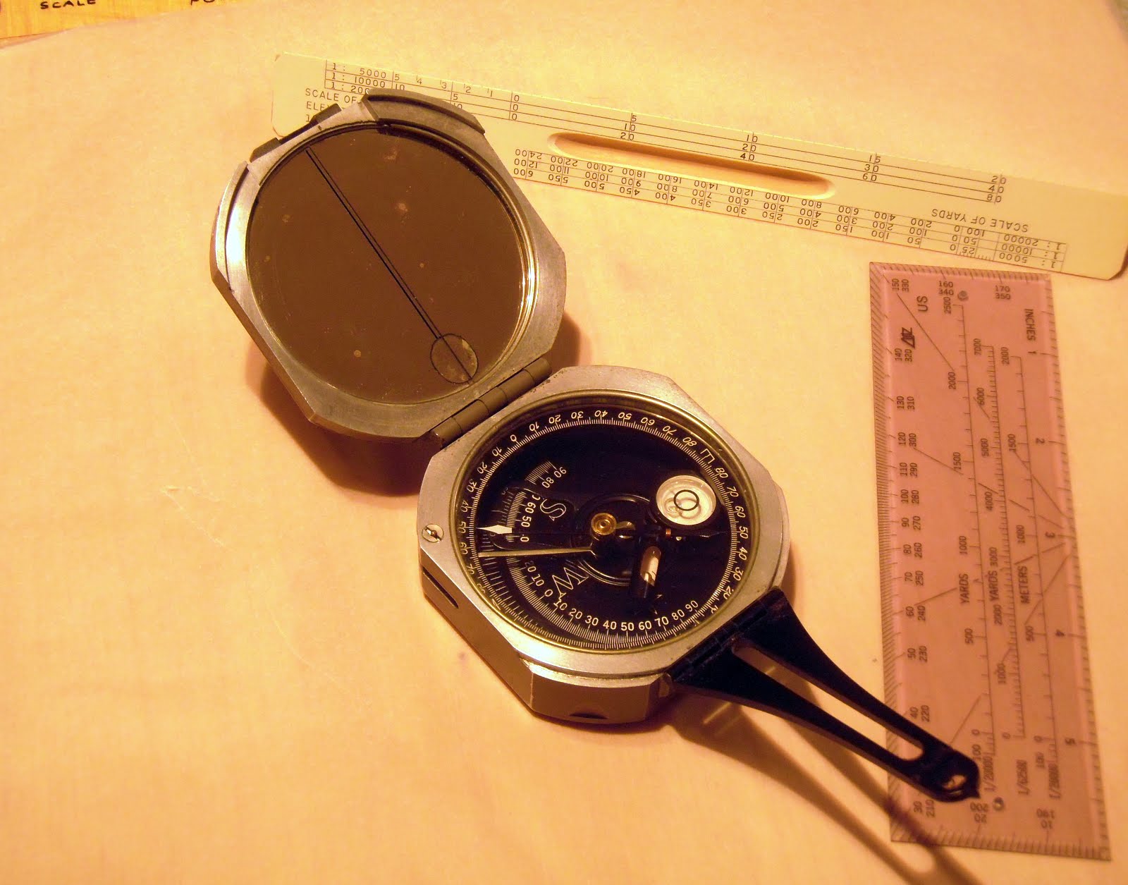
In 1765 the pair began work on the line westward, and this effort consumed the better part of the next three years. The survey party consisted of over 100 workers – axmen, Indian guides, surveyors assistants, hunters, runners, teamsters and general laborers. The work was both physically and mentally demanding. The effort required teams of axmen hacking a westward line of sight through virgin wilderness up and over the Allegheny Mountains, the survey team directing their clearing work using compasses that had to be checked almost daily for local variance (declination). Distances were precisely measured using survey chains or rods. At intervals Mason & Dixon would stop, set up astronomical observation stations and verify the line was on the same precise latitude as set at the Post mark’d West. Any necessary corrections to the line were made, north or south, depending on the results of the observations, and the survey continued westward. Following behind, teams of workers set heavy stone markers at one mile intervals and at five mile intervals specially engraved ‘crown stones’ were set, with one side engraved with the Calvert family coat-of-arms, the other with the Penn family coat-of-arms. On more than one occasion, after field checks revealed errors, crews had to go back and move the markers to their correct location.

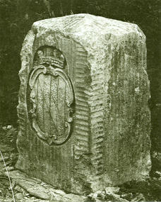
A crown stone marker showing the Calvert coat-of-arms

The original survey was supposed to run five degrees of longitude (265 miles) west from the Delaware River to fix the western boundary of the colony of Pennsylvania, but at the 233 mile point the party’s Mohawk guides called a halt. They had reached the western-most limit of the agreement for the survey set with the chiefs of the Six Nations and would go no further. Mason and Dixon realized that, for now, the survey had reached its end. At the 233 mile point they set a stone pyramid to mark the end of the survey and headed east to Philadelphia to analyze their results and prepare their reports.

In the summer of 1768 Mason and Dixon delivered 200 printed copies of their maps, survey data and final report to the project’s commissioners. The Calverts and the Penns accepted the results of the survey and the boundary between the colonies was formally recognized. It wasn’t until after the American Revolution, in 1784, that the line was extended to the full five degrees of longitude, this time by two of America’s best astronomers, surveyors and instrument makers – David Rittenhouse and the remarkable and indispensable Andrew Ellicott.

Sadly, Mason and Dixon never worked together again. In 1773 Jeremiah Dixon was elected a fellow of the Royal Society and he soon retired to his native Cockfield a wealthy and well respected gentleman surveyor. He died young in 1770, unmarried and with no heirs. Charles Mason continued to work for the Royal Observatory and its new Astronomer Royal, the Reverend Dr. Nevil Maskelyne. But Dixon became disillusioned with his work in England and lack of recognition for his continued contributions to astronomy. Nevil Maskelyne was well known as a ‘glory hog’ who often refused to give credit and recognition to others contributing to projects under his direction. While working on the boundary survey Mason had become good friends with many American scientific luminaries such as Ben Franklin and David Rittenhouse. Mason likely figured his talents would get more respect in the former colonies. In early 1786, while in bad health, he sailed again for Philadelphia with his wife and eight children. On arrival he communicated briefly with Benjamin Franklin but died in late October 1786 and was buried in the Christ Church cemetery in Philadelphia.

Mason and Dixon’s work on the boundary line was recognized in its time as an outstanding scientific achievement. In the mid-18th century the science of geodesy – the study of the shape of the earth – was in its infancy and there were a lot of unanswered questions. The best minds of Europe, particularly in France and England were turning their efforts to developing a better understanding the size, shape and form of the earth. At the time the best ways to work out these questions was to study closely the detailed results of ‘great arc’ surveys – highly accurate surveys that covered great distances. In 1830 the first great leap in applied geodesy occurred when Astronomer Royal George Airy published the first accurate spheroid of the Earth. A spheroid is a mathematical definition of the size and shape of the earth, and an accurate spheroid definition is the foundation on which accurate mapping and surveying is built. To calculate his definition Airy used multiple ‘great arc’ survey results provided by British, French, Russian and German scientists, but the only great arc survey he used to define the Western Hemisphere was the boundary survey conducted by Mason and Dixon some 70 years previously.

Good work stands the test of time, and Mason and Dixon’s survey remained one of the most accurate boundary surveys conducted in the Americas well into the 20th century. Even today surveyors using modern GPS-based systems marvel at the accuracy and precision these mid-18th century surveyors achieved. So the next time you cross the state line between Pennsylvania and Maryland remember the two geniuses who’s colonial-era work to settle an argument over a property line ended up helping to accurately define the shape of the planet we live on.

– Brian

Post script – as with so many of my posts on this blog, I stood on the shoulders of giants while writing this one. There’s a lot of good material covering Mason and Dixon’s boundary survey available on the web. John Mackenzie of the University of Delaware has published perhaps the best one page history of the survey available on the web (although his essay ends up wandering into territory I think should have been saved for a separate posting). But the story of the boundary survey and Mason and Dixon’s efforts really needs a book to cover fully and adequately. We are fortunate that Edwin Danson has written a wonderful volume that covers the background on the survey and a full accounting of Mason and Dixon’s work. Danson’s book is titled ‘Drawing The Line‘ and in my mind it stands with other modern classics of popular science history like Dava Sobel’s ‘Longitude’ or John Wilford Noble’s ‘The Mapmakers’ as a must read for anyone interested in the topic.

Perrysburg Plat Map

Posted on June 21, 2015 by Brian Haren

As I’ve mentioned in earlier blog posts, you can find interesting map in the most unusual of places. Earlier this month I was up in northwestern Ohio visiting with my father and decided to take a few hours and check out the local history. I found myself in the delightful town of Perrysburg, right across the Maumee River from my hometown of Maumee. Perrysburg and Maumee ‘grew up’ together during the 1800’s and for much of their history were economic rivals, vying for the lucrative trade that moved up and down the river. In the end both lost out to Toledo, situated a few miles downriver where the Maumee empties into Lake Erie.

Perrysburg became what can best be described as bucolic, a sleepy little town that time and development passed by until one day about 40 years ago folks recognized that the town had a charm and a unique history unsullied by commercial development and tract housing. Suddenly Perrysburg became a trendy place to live and visit. The city worked hard to retain the unique flavor of the historic downtown, and they’ve done a great job.

The town was first established in 1812 on a bluff overlooking the Maumee River. In 1816 two US government General Land Office surveyors, Joseph Wampler and William Brookfield, laid out the town street pattern. Soon after the residents decided to change the town name to Perrysburgh to commemorate Commodore Oliver Hazard Perry’s victory over British naval forces at the Battle of Lake Erie at Put-In-Bay. The ‘h’ was eventually dropped from the Perrysburg town name at some point lost to history.

Wampler and Brookfield appear to be some of the first government surveyors sent into what was known as the Northwest Territory after the War of 1812 to conduct official land surveys using the Public Land Survey System otherwise known as the township & range layout.

The federal government was eager to get this land surveyed, platted and sold. At the time land sales were a major source of revenue for the cash strapped US treasury, plus the government wanted to encourage settlement in the area to solidify American claims to territory ceded by the British and Native Americans under the Treaty of Ghent which ended the War of 1812.

Both Wampler and Brookfield were very competent surveyors and there are records of their work in both the National Archives and the state archives of Indiana, Ohio and Michigan. Wampler is cited by several sources for his efforts in correcting the sloppy work of other surveyors, particularly his work to establish two initial points for the Michigan surveys. Brookfield seems to have headed west from Perrysburg and eventually became a surveyor and later circuit court judge in St. Joseph County, Indiana.

What we don’t know is what induced these two gentlemen to lay out, or plat, the town of Perrysburg. Platting towns and settlements was not something surveyors in the employ of the GLO (General Land Office) did. My guess is that Wampler and Brookfield got specific instructions from the GLO to execute the survey after the town’s leading citizens petitioned their representatives back in Washington, D.C. How rare was it to have GLO surveyors plat a town? Well, there’s only four cities or towns in the United States that were platted by surveyors directly employed by the federal government. Perrysburg is one, Washington D.C., Croghansville (Fremont) Ohio and Shawneetown in the Illinois Territory are the others.

The notation in the lower right corner indicates that the plat was accepted into the General Land Office records on 18 March 1817 by Josiah Meigs, the Surveyor General of the United States. In 1816 the river was called the Miami River after the Miami Indian Tribe that inhabited the area

The layout and street pattern of Perrysburg as shown in the 1816 plat is still visible today on maps and aerial images. In fact, little has changed. Some lots have been combined, particularly along Louisiana Avenue, which became Perrysburg’s main street and commercial district, and some rail lines and secondary roads have intruded. But for the most part downtown Perrysburg is as Wampler and Brookfield laid it out almost 200 years ago.

To see just how little has changed in the old section of Perrysburg click on the image below to launch a web map that lets you compare 1816 to 2015. Have fun!

– Brian

Calculators

Posted on September 7, 2014 by Brian Haren

The topographic sciences are a math intensive endeavor. Map making is far more than drawing squiggly lines on a sheet of paper. Before those squiggly lines get drawn there first must be a determination of things like the geographic extent of the map, the scale, the coordinate system and projection and the precise location of key features on the map. This all has to be figured out before the first line is drawn. This means number crunching, lots and lots of number crunching. A competent topographer needed to be conversant in everything from plane geometry to matrix algebra to calculus.

Today all of the complex math involved in map making is easily and swiftly handled by computers. A mouse click or two in a multi-threaded 64-bit desktop application launches a routine that returns a mathematical solution in seconds. But just 60 years ago the same routine would take a competent topographer or mathematician hours to calculate by hand and would involve the use of special forms, books full of mathematical tables, slide rules and, if he or she was lucky, a hand cranked mechanical calculating machine that might be able to hold precision to a decimal place or two.

There was a time not long ago that the accuracy of these calculations was so important that the job of ‘calculator’ was something that a young man or woman with good math skills could make a decent living at. For example, in the US Geological Survey (USGS) the topographic or geodetic survey crews would collect the data in the field and do some initial accuracy checks just to make sure they hadn’t ‘busted’, or obviously exceeded the required accuracy for the type of survey the were conducting. All the data would then be sent to a USGS field office or headquarters where the specially trained ‘calculators’ would re-evaluate the data to provide a final approved result.

About 40 years ago there was a paradigm shift in the topographic field that was brought about by the introduction of (relatively) inexpensive handheld calculators. It’s hard for those who didn’t live through this time to understand just how big of an impact the handheld electronic calculator had on the scientific and engineering world, and this included the topographic sciences. My father was (and still is!) a chemical engineer, and I remember watching him sit at the table after dinner grinding through stacks of engineering calculations with a slide rule and long calculation sheets. One day in the mid-1970’s he went out to the local J.C. Penneys and came home with a new device that fundamentally changed how he worked – a simple ‘4-banger’ Texas Instruments calculator, probably the TI-2500 ‘Datamath’ model. All it did was add, subtract, multiply and divide (hence the ‘4-banger’ designation) and at $119 dollars (equivalent to $575 today) it was a significant investment, but the improvement in accuracy and speed of calculations made the investment worthwhile.

Texas Instruments TI-2500

From there things only got better. While desktop computers were still just pie-in-the-sky devices we saw on the weekly episodes of Star Trek, handheld calculators quickly started dropping in price while adding newer and more advanced features. Faster and cheaper processors, better displays, better batteries, storage registers (i.e., memory), statistical functions, angular calculations, exponent calculations, continuous memory, programming, symbolic equations, alpha-numeric registers, unit conversions and a lot more. By the time I started college in early 1975 I could pick up a feature rich Texas Instruments scientific calculator like the SR-50 for a little over $50. This calculator offered all the capabilities a financially and academically struggling student needed for most of his college career.

In the early 1970’s a new player emerged onto the calculator scene. Hewlett-Packard (HP) was a highly regarded electronic test equipment and computer manufacturer that had released some very successful desktop calculators and mini-computers in the late 60’s and early 70’s. One of the company’s founders, Bill Hewlett, was watching the emerging calculator market and challenged his engineers to come up with a calculator designed specifically for scientists and engineers that would fit into his shirt pocket. Even though HP’s marketing group didn’t think it would sell, Bill pushed the project forward and in 1972 HP released the HP-35. It took the scientific and engineering world by storm. The marketing gurus said HP would never sell more than 10,000 units, total. In the first year alone HP sold over 100,000 and when production of the HP-35 ended in 1975 it had sold over 300,000. That’s pretty impressive sales numbers for a calculator that cost over $2,000 in today’s dollars!

The HP-35 Scientific Calculator

The HP-35 set the standard for all HP calculators that followed. Rugged construction, high reliability, excellent documentation and support, well implemented features and the unusual but very efficient computational system known as Reverse Polish Notation (RPN).

As a young college student I was well aware of HP’s offerings. The calculators were offered for sale in the college bookstore where I was studying and HP ads were appearing in a lot of the magazines I regularly read (like Scientific American). In addition, HP would ship you large envelopes stuffed full of promotional material and copies of the company’s magazine devoted specifically to it’s calculators and their use. At the time my brother worked at a test lab in Toledo, Ohio and would bring home one of the early HP-21’s that the lab owned just to play with. I was hooked, but there was no way a poor college kid was going to be able to afford a calculator that cost at least four times what my Texas Instruments calculator had cost me.

Fast forward a few years to 1982 and I’m out of college, in the Army Corps of Engineers and reporting to the Defense Mapping School at Fort Belvoir, Virginia, to attend the Mapping, Charting and Geodesy Officer’s Course (MC&GOC). On the first day the course leader handed each of us an HP-31 calculator and gave us a fast course in Reverse Polish Notation and stack manipulation. Then it was off to the races, with the first part of the course covering survey theory, statistics, matrix algebra and least squares. Since the Army was paying me a little extra each week to attend the class I figured it was time for me to buy my own HP calculator. One Saturday morning I took the Metro to an office supply store in downtown DC and bought myself a brand spanking new HP-32E.

HP-32E

That purchase triggered several decades of HP calculator accumulation. I can’t claim that I ‘collect’ HP calculators since I rarely go looking for them. However, if one happens to fall into my lap – usually from a co-worker looking to get rid of an old unit or I stumble on one in a pawn shop or at a yard sale – I’ll pick it up and add it to my stash.

I’m sure some of you are asking yourselves, “But does he still use any of those calculators?” You bet! While high end GIS software and spreadsheet programs have taken over most of the heavy number crunching I do, I still keep a modern HP 35S, on my desk for those ‘right now’ calculation needs that crop up almost daily. In addition I run HP calculator emulators on my iPhone and Android devices that have proven themselves very useful when in meetings and someone needs quick averages run on a series of numbers, or some quick sums done, or a rough comparison between estimates calculated. The handheld calculator is still a very useful tool!

Let’s take a look at a few calculators in my collection and discuss their significance:

Texas Instruments TI-59

This is one of the few non-HP calculators in my collection, but it’s here for two reasons. First, this particular calculator used to belong to my father, who used it in the latter stages of his professional career.

The other reason I include it is because it represents an interesting example of how technology advances regardless of what the powers-that-be want. In the early 1980s I was attending the Air Load Planners School at Fort Bragg, where we learned to do aircraft load and balance configurations for our unit’s wheeled and tracked equipment. A couple of my classmates were out of the Field Artillery battalions on Fort Bragg and all were using TI-58 or 59 calculators. During a break one day I asked them where all the TI calculators came from. They told me that the calculators actually belonged to their units and were used as unofficial (and unapproved) replacements for the big, bulky FADAC computers the Field Artillery units used to calculate indirect artillery fire. The FADAC was 1960’s technology that took up an entire table, required a 10 kilowatt generator to power and cranked out enough heat to fry an egg. In the early 1980’s some sharp young lieutenants at the Field Artillery School figured out that all the computations the FADAC system did could be easily handled by the TI-59. Since the TI-59 was one of the earliest magnetic strip programmable calculators it was easy to copy all the calculation routines to the strips and share them around. Local Field Artillery units snuck out and locally purchased TI-59 calculators and began using them in place of the FADAC systems. This was particularly advantageous for light artillery units in the 82nd and 101st Airborne Divisions since they could carry ‘FADAC-lite’ capability in their rucksacks.

HP-41CV

The HP-41 calculator was out of this world – literally. More on that in just a bit.

When HP introduced the HP-41 in 1979 it appeared to make all previous HP models obsolete. Not entirely true, but that’s the impression it gave. A lot of engineers and scientists chucked their old calculators, took out loans and bought themselves an HP-41 and accessories. Many of those calculators are still chugging along and their owners refuse to let go of them or move up to something more advanced. What made the HP-41 so good? It wasn’t HP’s first programmable calculator, or its first with continuous memory. What made the HP-41 special was that it was the first handheld calculator with an expansion interface. When you bought the HP-41 you were buying just one component of a larger system that could include dedicated expansion modules for things like surveying, electrical engineering, structural analysis or celestial navigation. You could hook it up to a floppy disk drive to write or retrieve data. You could attach a bar code reader or send your work to a printer via an infrared link. You could hook it up to sensors to monitor temperature, humidity, blood pressure, and lots more. The HP-41 was also HP’s first calculator that used an LCD display, greatly reducing battery drain, and it introduced the idea of alpha-numeric tags for programming. In short, the HP-41 was more computer than calculator.

The HP-41 caught on strong with the surveying community and a lot of third party surveying applications were developed for it. Many of these calculators went to the field with survey crews and computations were run on the spot to verify collected data. The HP-41 provided the first glimpse into the future, where theodolites and computers would become integrated systems and all data collection and reduction was done on the instrument in real time.

This particular calculator obviously doesn’t work, and it’s damaged beyond repair. I picked it up in my unit in Germany back in 1998. We were doing a final clean-out of unserviceable equipment left behind from the inactivation of the 649th Engineer Battalion (Topographic) and I found this calculator in a box that was headed for the dumpster. I saved it only because it had someone’s name on the case and because I didn’t have an example of an HP-41 in my collection, working or not. So, Surveyor Howse, if you want your HP-41 back just drop me a line. I’ll be happy to return it!

Now, what about the ‘out of this world’ comment? Well, in 1980 NASA went looking for a programmable calculator that could be carried by the astronauts on the first Space Shuttle flight. The idea was to program the calculators with critical flight data and routines for the astronauts to use in case Columbia’s on-board systems failed. Each of the two pilots, John Young and Robert Crippen, carried HP-41s in their flight suit pockets. This made the HP-41 the first handheld calculator in space. Thankfully the pilots didn’t need the calculators for their intended purpose, but HP-41s flew on a number of subsequent flights, mainly as auxiliary computers to help take the computational loads off of the Space Shuttle’s overburdened computers. One of these HP-41s, used by Astronaut Sally Ride, is on display at the National Air and Space Museum.

HP-34C

The HP-34C is perhaps the best example of HP’s third generation of handheld calculators, and in its time was considered HP’s high end keystroke programmable calculator. None of the third generation calculators offered card reader capability like the HP-41 or HP-67, but with continuous memory capability you could key in a wide variety of short programs and run them as needed. This calculator also sports what is considered the classic HP calculator key layout, and it’s a layout that is still praised today for it’s clarity and ease of use.

HP-11C

The HP-10 series of calculators came out in 1981 and included the 10C, 11C, 12C, 15C and 16C. Of this group the 11C and 15C Advanced Scientific calculators were by far the most popular, and the 11C remained one of HP’s best selling calculators for years. In my office there are still civil engineers with old, battered, but functioning 11C or 15C calculators on their desks.

Both of these calculators are 11C models. The one on the bottom with the missing HP sticker has an interesting history. This is the second HP calculator I bought for myself, back around 1983 (not long after buying my HP-32E). I decided I just couldn’t live without continuous memory. This calculator was carried daily, usually in the cargo pocket of my Army BDU uniform. One day I came home from work and my lovely wife met me at the door holding a wet pair of BDU trousers that she had just pulled out of the clothes washer. She looked at me and growled, “It ain’t my fault!” and tossed me the trousers. I knew right away she was referring to something I had left in the pockets but didn’t know what. As I squeezed the various pockets I immediately felt the outline of my 11C and knew I was in trouble. I pulled the calculator out and was disappointed, but not surprised, to see it wouldn’t turn on. I figured I had nothing to lose by trying to resuscitate it, so I pulled out the batteries, wiped it down as best I could and put it in a nice dry location. A few weeks later I popped in a new set of batteries and hit the ‘ON’ button. To my amazement it came to life! I ran through all the built-in diagnostic utilities and it returned no errors. The calculator returned to work with me the next day.

Somewhere along the way this calculator went missing. At the time we were living in Frankfurt, Germany so I went down to the big Herite department store on the Hauptwache and purchased a new one (complete with German documentation). That calculator (the one on the top in the picture) is still running on the original set of batteries I installed in 1985! About a year later I was going through some old papers from work and was surprised to find my old, original 11C stuffed into a manila folder full of forms. It must have gotten accidentally dropped into the folder without me noticing it. So now I have two 11C’s, and both work like champs!

HP-32S (left), HP-42S (right)

This series of HP calculators was introduced in 1986 and was intended to replace the 10-series discussed above. Mostly they succeeded. The HP-32S remained in production for over 10 years and was actually quite a good yoeman scientific calculator. Nothing spectacular, just a very reliable, rugged calculator loaded with useful features. Its dot matrix display made it a bit hard to read in some lighting conditions, but it made better use of the built-in alpha-numeric register options.

The HP-42S is an interesting product. In 1988 the venerable HP-41 was reaching the end of its product life cycle and HP had plans to phase it out in favor of the new HP-48 series of graphing calculators. Yet HP knew that the HP-41 series had a strong, almost cult-like following and that HP-41 users would be reluctant to abandon their existing applications and programs. In an effort to bridge the gap between the HP-41 and the newer HP-48, Hewlet Packard introduced the HP-42S. Basically they ported the HP-41 ROM over to this new format and incorporated some improvements – faster processor, better display, more storage registers and a few other upgrades like a matrix editor. At first the user community took it as a joke – an HP-41 ‘compliant’ operating system on a calculator that offered no input other than keystroke programming and no output other than an infrared link to a printer. Sales were slow, and while HP kept it in production for about 7 years it never really sold well. Can you tell where this is going? Now, more than 20 years after its introduction the HP-42S is a hot collectors item. HP aficionados now recognize it as something special – a ‘hot-rodded’ version of their beloved HP-41 in a smaller and easier to use package.

HP-48G Series

Let’s wrap this up with a look at what many (including me) consider to be the last of the classic HP calculators. The HP-48 was developed to replace the HP-41 series, and fully succeeded in that goal. While the HP-48’s never developed the devoted following the HP-41 series did, the HP-48 succeeded on another level – they became solid and serious workhorse calculators that found their way into a wide range of applications. They were well built, feature rich, expandable, offered great battery life (using commonly available AAA batteries) and excellent connectivity with a wide variety of devices via a standard serial cable. Survey program developers quickly took advantage of the HP-48’s power and capabilities and wrote software that turned the units into data collectors that hooked right up to early digital theodolites, making the HP-48 one of the first dedicated data collectors on the market. The calculator shipped with its own application library installed, but developers wrote hundreds of additional applications covering a wide range of subjects such as biodiversity evaluation and commercial aviation fuel load calculations. One of the HP 48’s in my collection was surplussed out of the University of Michigan Dept. of Physiology where it was used as a human bio-metric data controller. The HP-48 stayed in production for 13 years making it one of the most successful lines of calculators produced by any manufacturer. Today there are thousands still in use around the world and, like the HP-41 a generation earlier, their users refuse to let go of them.

Sadly, after the HP-48 Hewlett-Packard all but abandoned the calculator market. HP management and marketing folks didn’t see any future for handheld calculators and let the calculator unit wither on the vine. Calculator development was moved off-shore and HP’s offerings became little more than bland re-badged products produced in China. For a time HP even toyed with abandoning its signature RPN operating system in an effort to capture a share of the student calculator market dominated by Texas Instruments.

HP’s interest in calculators seemed to perk up a bit as the 35th anniversary of the HP-35 approached. In 2007 they introduced the HP-35S, a design that received a lot of input from classic HP calculator aficionados. It was a good effort that hearkened back to the classic HP calculator designs of the 1980s and runs a faithful implementation of HP’s classic RPN operating system. Since then not much has happened. Two years ago HP released a new product called the HP Prime, a high end graphing calculator that gets very good reviews, but today HP’s serious scientific calculator offerings can be tallied on the fingers of one hand.

Let’s hope we are not seeing the end of a long and storied calculator dynasty.

– Brian

To The Corps!

Posted on July 7, 2014 by Brian Haren

I spent most of my military career serving either as a Topographic Officer (21C) or a Terrain Analysis Warrant Officer (215D) in the Army Corps of Engineers. It was clear throughout most of my career that the Engineer branch really didn’t know what to do with us. Longstanding US Army doctrine said that the Corps of Engineers ‘owned’ the topographic and terrain analysis (military geography) discipline, but owning and effectively managing are two different things. The field was so small and specialized that the Engineers tried to manage it by exception, as though we all carried a pox that would infect ‘real’ Engineers if we came too close.

However, this was not always the case. For several decades in the first half of the 19th century two military engineer organizations ran parallel to each other in the US Army. One organization was filled with officers with mostly limited engineering backgrounds. This group was detailed to handle general engineering support to field units, tackling simple engineering tasks like improvements to local fortifications, managing the construction of tracks and trails in support of military movement and doing local reconnaissance and field sketching in support of military operations. These were the regular Engineer forces assigned to the field Army. The other group was filled with the cream of the graduating classes from West Point and some of the top graduates of the few engineering schools operating in the US the time. This group handled most of the civil works improvement projects along the coastlines and interior waterways and mapped the new western territories and opened them for exploration and settlement. This last group truly was the civil engineering force for the new nation and was known as the Corps of Topographical Engineers.

Uniform button design for officers assigned to the Corps of Topographical Engineers.

From roughly 1812 to 1863 the Corps of Topographical Engineers operated as an independent organization, sometimes as a separate branch within the War Department, sometimes as a wholly autonomous section within the Army Engineers. The ‘Corps’ was little more than a roster of officers detailed to the Topographical Engineer branch. There were no enlisted personnel assigned and Topographical Engineers were usually dependent on local Army commanders to provide the needed manpower for projects.

What the Corps of Topographical Engineers did have was some of the best civil engineering minds in the nation. At a time when trained engineering expertise was hard to come by – civil engineering as a defined discipline wouldn’t emerge until well after the Civil War – the Army and Congress often turned to the Corps of Topographical Engineers to handle most of the early public works planning and management. Topographical Engineers explored and mapped the Great Lakes region, managed canal construction and waterways improvements and even surveyed and planned lighthouse locations. In the 1850s, when the federal government needed to have the lands acquired from Mexico and the newly incorporated State of Texas explored and mapped, they sent in the Topographical Engineers. When Congress needed to know if there were suitable routes through the Rocky Mountains for the planned transcontinental railroad they sent the Topographical Engineers to have a look. Once the Oregon Territory dispute was settled with England the Topographical Engineers moved in to map the rugged interiors of what is today Oregon, Washington and Northern California.

Regulation on how officers assigned to the Corps of Topographical Engineers are to be detailed, or appointed, to duties. Excerpted from the ‘Army and Navy Chronicle’, January 2, 1840

In 1863 the Army folded the Corps of Topographical Engineers into the regular Corps of Engineers and a proud organization that provided immeasurable service to the nation disappeared. I guess it was inevitable since there was a desperate need for trained Engineer officers to support the Federal armies during the Civil War, and there was growing overlap in the roles of the two organizations.

The Corps of Engineers’ love affair with it’s mapping and surveying mission waxed and waned over the next 150 years. Engineer officers still found themselves assigned to important topographic missions as America settled it’s western territories, rushed to map its newly acquired territories after the Spanish-American War, threw armies across the seas in World Wars One and Two and stared down the Soviets during the Cold War. I believe the peak of the Corps of Engineers interest in and dedication to its topographic mission came with the establishment of the Army Map Service in WWII. The Engineers realized they had to get damned serious damned fast about this mapping thing and developed the doctrine, equipment, techniques and technology necessary to produce maps and related products to support a world-wide war effort. This effort continued well into the Cold War, and it was the Army Map Service (and later the Army Topographic Command) that gave us groundbreaking developments such as the Universal Transverse Mercator grid system, the Military Grid Reference System and early research work on an earth-centered geoid that ultimately became WGS 84.

As the Cold War wound down the Corps of Engineers interest in its mapping mission wound down too. As more and more map production was pushed to the national level (to the Defense Mapping Agency, which became the National Imagery and Mapping Agency, which became the National Geospatial-Intelligence Agency) and mapping systems moved from paper to digital and became embedded in battlefield command and control systems, the Engineers seemed on a headlong march to shed their traditional topographic role. Inevitable? Perhaps. Wise? I don’t think so. Topographic knowledge is the foundation of military expertise. Great generals like Napoleon, Lee and Grant, and Patton all talked about the necessity of being able to visualize the battlefield, the ability to identify ‘good ground’. Someone will always have to paint the battlefield picture for the generals, and that’s the job of the Topographic Engineer.

Although the Corps of Topographical Engineers has faded into history they are not forgotten. There is a small but active group that keeps the history of the early Topographical Engineers alive through research and reenactments. They are the U.S Corps of Topographical Engineers. Their website is a great resource for anyone interested American history and the story of how America grew in the early 19th century.

U.S. Corps of Topographical Engineers historical website

So here’s to the Corps! To a group of dedicated Topographical Engineers that explored, mapped and helped build this great land. Ladies and gentlemen raise your glasses.

To the Corps!

– Brian

Topographic Instructions of the US Geological Survey

Posted on May 18, 2014 by Brian Haren

How do you make a map? More precisely, how does one produce a map compiled to specific standards for accuracy, content and style? Does that question keep you up at night? Nah, me either. But it is an interesting question and I’d bet that if you put it to 100 people you’d get 110 answers.

Of course today it’s easy. Nobody really makes a map these days. Most just go to Google Maps on their smartphone or tablet, and these days that’s about all the ‘map’ most people want or need.

But 100 years ago things were much different. Back then there were still vast unmapped areas of the US and it was the responsibility of the US Geological Survey (USGS) to send topographic parties in to map them. This was before the era of cell phones, internet, GPS and even radio communications. Checking with the home office involved the US Mail or, if they were lucky, telegraph. For that reason these parties operated autonomously under the direction of a Party Chief. The Party Chief was part military general, part football coach and part college professor; he ruled with an iron fist and made sure everything was run properly, was responsible for the motivation and morale of his party and was the brains of the outfit. The Party Chief was vested with enormous authority because he had an enormous responsibility – he answered to his regional Chief Geographer for the accuracy and quality of his party’s work.

In 1913 Party Chiefs didn’t go about their work blind. They operated under a very detailed set of instructions and standards laid out in a USGS publication titled Topographic Instructions of the United States Geological Survey.

I find this a fascinating manual because it is the only publication I’ve seen that lays out in detail the steps necessary to create a map from scratch. It covers all the processes involved in creating a map to very specific accuracy, content and composition standards. This is, quite literally, the document that defined what we know today as the standard USGS topo quad sheet. Of course the USGS was producing standard topo sheets before this manual was published, but indications are that prior to 1912 the instructions were covered in separate publications and broken out by discipline. This manual brought it all together in a single reference that is remarkably clear and concise for its time, stripped of a lot of the superfluous language that Edwardian-era government functionaries were so fond of using. This is a manual designed to be used in the field by men who have a job to do.

The topics covered include

primary and secondary triangulation
primary and precise leveling
plane table surveying
map construction (compilation), drafting and editing
instrument care and repair

But beyond the technical, Topographic Instructions of the United States Geological Survey covers detailed administrative instructions to Party Chiefs on topics like crew selection, first aid for pack animals and crew members, how much food to pack, how many fountain pens to bring along, how to set up a base camp, even how to interact with local officials and the press.

It’s a soup-to-nuts manual on how to make a map from scratch.

– Brian

Neatness Counts

Posted on March 27, 2011 by Brian Haren

Earlier we discussed the use of field notebooks and the lost art of field note taking. I fear that neat, disciplined and structured field note taking is a lost art in the today’s world of texting, instant messaging, and email. Even in the engineering, surveying and topographic field (where I work) the use of field notebooks appears to have been brushed aside by smartphones, laptop computers, data collectors and the assorted electronic bric-a-brac that has come to dominate the field. And yet – and yet – all this powerful technology still leaves us with critical information gaps. The problem is not so much that people aren’t writing stuff down, it is that they are writing it down in formats that are so very disjointed, disconnected and perishable. An email here, a quick scribble on a random notepad there. It gets lost or never gets integrated into the project file. Months or years down the line engineers and maintenance personnel are left to wonder just where something was placed or how it was constructed because the story of that project was not properly documented.

Now, I’m not implying that the use of field notebooks will solve all of these problems. Field notebooks are not a panacea for lousy project management. My point is really that disciplined and structured note taking should be viewed as a key skill – and a requirement – for surveyors, engineers, topographers and other key staff. Of course the ideal place to write all this down is in a field notebook, a field notebook that gets turned over to the organization, copied, indexed and integrated into a document management system at the completion of the project.

Neat, disciplined, complete and structured note taking. Just what does that mean?

The disciplined and complete parts are easy. Notes need to be made on any issue, topic, observation or discussion that directly impacts a project. It is really nothing more than getting in the habit. Get in the habit of having your notebook with you and writing stuff down. Complete means get it all down. Think of each record you create in the notebook as a miniature story – it needs to have a beginning, a middle and and end. What you observed, when and where you observed it, what was important about it, who was there, what was agreed to, what conclusions were reached and, if necessary, sketches or diagrams that are key to the issue at hand. Make it a complete story!

Neat and structured are two somewhat subjective concepts. Everyone has their own style of organization and handwriting. The important thing is to make it neat, legible and logical in structure. Always remember that the intent is to make it easy for you and others in your organization to reference in the future. How far into the future? I routinely reference survey records for the airport I work at that are 60+ years old. The neatness and structure (and completeness) of those records allow me to rely on them for locating structures and utilities that were abandoned and forgotten about decades ago.

I can only offer suggestions for the concepts of neatness and structure. As I mentioned in my earlier post, field note taking used to be a topic taught in all beginning surveying and civil engineering courses. Colleges, universities, government agencies (like the USGS and the USC&GS) and even individual companies used to have their own field note format requirements. Some agencies, like the US Army Corps of Engineers, would even have entire bound books printed with pre-formatted pages.

A few agencies still provide specific field note standards. Surprisingly, most are state departments of transportation (DOT). For example, the Oregon DOT, provides specific guidance for field note structure. Their Survey Field Note Standards (October 2006) provides very specific field note examples. The same for the Montana DOT. Their Survey Manual provides a chapter on sample notes that contractors are expected to follow.

But since this is my blog and I love old stuff, particularly old stuff that still has relevance, we’re going to take a trip back to the 1950s. A time when cars had carburetors, space travel was the stuff of science fiction and real men did surveys with optical theodolites and steel measuring tapes, and wrote everything down in hard bound notebooks. A couple of professors at the University of Missouri put together a course in introductory surveying and field measuring. A large part of the class involved proper field note recording. This course was to serve as the foundation for all surveying and civil engineering instruction to come, so the instructors needed to make sure the students got started on the right foot with disciplined, accurate, structured and comprehensive field data recording. The two professors, Clarence Bardsley and Ernest Carlton put together a gem of a book titled ‘Surveyors Field Note Forms’.

Bardsley & Carlton, Surveyor’s Field
Note Forms (3rd Ed.)

The book opens with a treatise on the importance of field notes and the necessity of being an accurate, error free, neat and complete note taker.

“Allow no items for the memory; all facts should be on the record.”

“A good surveyor takes pride in the appearance of his notes. A neat-appearing, well arranged set of field notes commands confidence and builds prestige in the surveyor.”

“Field notes should be clear and convey only one possibly correct interpretation. Descriptions and narrative matter should be in acceptable English. Sketches should be drawn to approximate, or convenient, scales. All numerals indicating distances, angles, or elevation should be carefully formed. Particular care should be exercised in obtaining a logical order and sequence of all notes, for they should be absolutely clear and understandable to the student, other surveyors, computers*, or draftsmen.”

The book then goes on to provide specific examples of problems and how the field notes should be formatted (click on any image to open it full-size):

Length of Pace Measurement

It was once common practice for surveyors to regularly measure and record their pace count over various types of terrain (flat, hilly, uphill, downhill, etc.). Before accurate handheld measurement devices like GPS surveyors used pace count to do help them with tasks like finding property corner stakes or do rough fence line measurements.

Correcting for Horizontal Slope

Don’t you just love the name ‘Trachoma Hospital?

Using Rough Triangulation to Determine Distance

Although the equipment has improved, surveyors and engineers still use the principal of triangulation to determine inaccessible distances.

Sewer Stake-out

Construction stake-out, whether for sewers, buildings or roads, is still bread-and-butter work for surveyors.

Use of the Grade Rod

Field notes are for more than writing down numbers. Often the engineer or surveyor needs to write down a description of how a particular piece of equipment was used, or a methodology that might need clarification.

Height of Object

Again, the equipment may have changed, but the procedure is still the same.

Determining Azimuth From True North

Using solar or star shots is still an accepted practice for determining the relationship to true north.

The point of the above is not really what is on the page as much as it is the legibility, accuracy and completeness of the data. One hundred years from now, when Microsoft .pst files are lost to eternity, digital CAD files can’t be opened and survey data collector files are corrupted beyond recall someone will still be able to pull a notebook like this one off the shelf, open it and clearly understand what the author wrote and was trying to convey.

Neatness does count.

As I was wrapping up this blog posting I asked Roberta (5th Grade Teacher of the Millennium) if kids in grade school still get penmanship lessons. I was disappointed but not surprised to hear that, in her school system at least, penmanship has been sacrificed on the altar of computer skills. Apparently the school system feels that there is not enough time to teach and practice penmanship, and since kid are all wired up to computers these days the time ‘wasted’ on penmanship is better put to teaching computer and ‘keyboarding’ skills. How sad…

– Brian

(*Note – In the 1950s the term ‘computer’ meant something completely different. Back then a ‘computer’ was an individual who was responsible for doing final computations against the surveyor’s field notes and applying statistical methods to determine the accuracy of the survey results.)

Measuring Things

Posted on February 27, 2011 by Brian Haren

US Coast & Geodetic Survey leveling party working in Atlanta, 1927

In the olden days, like before GPS, before you could make an accurate map real men had to go out and measure things. This ‘measuring’ was called surveying, and it involved the extremely precise and accurate determination of the horizontal and/or vertical location of points on the ground known as survey control. This survey control establishes the accurate framework upon which a map is built. Horizontal measuring was called triangulation. Vertical measuring was called leveling.

The picture above comes from the US Coast & Geodetic Survey 1927 Seasons Report prepared by Captain E. O. Heaton (USC&GS). It shows a topographic leveling party at work in Atlanta. If anyone can figure out where in Atlanta these guys are working I’d love to know!

A few things to note. The fellow holding the umbrella is most likely a black local laborer hired to help the party haul equipment and provide general assistance. The umbrella he’s holding isn’t to keep the surveyor from getting sunburned – it is to protect the instrument from direct sun and prevent glare when sighting through it. To ensure accuracy survey parties often used umbrellas to shade their instruments and stabilize temperatures.

The fellow squatting is a surveyor who is acting as the recorder. He is writing down the readings being called out by the surveyor looking through the instrument. The recorder’s job was extremely important because he didn’t just write down what the surveyor called out, he would do on-the-fly quality control checks on the values the surveyor gave him to ensure they were staying within the accuracy standards established for that particular survey. If the recorder makes a single mistake, such as not catching an error in the surveyor’s observations or by writing something down wrong (like inadvertently transposing a number or putting a decimal point in the wrong place) he could lose an entire day’s work. In my experience you wanted your most meticulous guy and your best mathematician doing this job – perfectionists made good recorders. The recorder is writing his notes down in a bound hardback book known as a survey field notebook. That notebook would be turned in to the USC&GS at the end of the project and go on to become a part of the legal record of the survey. I have no doubt that very notebook still exists in the archives of the USC&GS now held by the National Oceanic and Atmospheric Administration. I’d love to take a peek at it!

(The job of recorder is one of those skills that has been replaced by computers. Today’s surveying instruments now automatically store the readings and calculate values internally. The computer integrated into the survey level lets the surveyor know via a digital display if the readings are within the specifications set for the job. It’s called digital leveling.)

But what is the surveyor looking at? Well, there are two people missing from this photo that make up the leveling party. The surveyor is looking through the survey level at a stadia rod being held by another party member known as a rod man. A stadia rod is a long pole marked off in feet and inches. Behind the surveyor is another rod man with another stadia pole (the location of the stadia poles is determined by the survey party chief and is based mainly on topography and the ability to see both poles from where the survey level is set up). The surveyor looks though the level and calls out the elevation mark he sees on the first stadia rod. He then reverses direction and calls out the elevation he views on the second stadia rod. The difference in numeric values he views on the two stadia poles is the difference in elevation between them:

Click on the image to open full size

Additionally, if this is a simple differential leveling job (and I think it is based on the type of level being used), there is another crew of chain men measuring the distance between the two stadia rods. In 1927 this would have been done using steel survey tapes or chains.

Leveling is slow, tedious and physically demanding work. There were no old farts out working on leveling parties except perhaps as party chiefs. The rod men and the chain men were constantly moving, carrying the survey forward. The instrument man and the recorder were responsible for moving and setting up the level in a new location, and the party chief was moving between all members of the survey party and scouting ahead for new setup locations.

Their work was absolutely critical, though. The meticulous work of the surveyors of the US Coast & Geodetic Survey and the US Geological Survey created the accurate spatial framework that this countries maps and charts continue to be built upon.

But that’s not the end of this story! I got interested in this picture for a particular reason. The vertical survey control for the airport I work at was established by this particular USC&GS survey project. I would like to think that it was these three unnamed gentlemen who, sometime in 1927 or 28, ran their traverse down into College Park, GA and set the single elevation benchmark that became the origin point for all vertical survey work done at the airport until the advent of GPS-based survey in the late 1990s.

Brian

Inter-American Geodetic Survey

Posted on January 23, 2011 by Brian Haren

The Inter-American Geodetic Survey (IAGS) was one of those extremely successful, yet little known, US Army (and later, Dept. of Defense) programs established after WWII.

The IAGS was created specifically to assist Latin American countries in surveying and mapping their vast internal regions that were either poorly mapped or entirely unmapped. The IAGS was established in 1946 as part of the Army Map Service and was headquartered at Fort Clayton in the Panama Canal Zone. The Army Map Service set up a complete survey, cartographic and map reproduction school at Fort Clayton and over the next 30 years trained thousands of military and civilian personnel from most Latin American and Caribbean countries. Attendance at the IAGS school at Fort Clayton was seen as right of passage for many up and coming officers in Latin American militaries, and it was common to run across senior officers – colonels and generals – from South American countries who talked fondly of their time spent at Fort Clayton, taking surveying or cartographic classes (one infamous graduate of the IAGS schools just happens to be Panamanian dictator Manuel Noriega, who attended the cartographic school in the 1960s).

The IAGS didn’t just provide training. It also provided the equipment and personnel to assist the participating countries in establishing their own self-sufficient mapping and surveying programs. The goal was to provide the training, equipment and technical support but have the individual countries take over their own mapping efforts.

Now, I’m not going to pretend that the IAGS was all altruistic good-will on America’s part. We learned the hard way during WWII that many Latin American countries were at best reluctant allies, at worst active sympathizers with the Nazi regime. At the end of WWII the political systems in these countries ranged from shaky democracies to hard line dictatorships. The US Government became concerned about the effects of political unrest and Communist influence in the region, and instituted a number of programs designed to bring Latin America firmly under American influence and to foster democratic principles and improve economic conditions. The IAGS was just one of many programs created as part of this effort. One extremely important benefit the IAGS provided back to the US was that we were able to get American personnel on the ground in these countries to make detailed evaluations of local conditions (after all, that’s what surveyors and cartographers do, right?) and we got maps that were created to US standards for vast areas of Central and South America.

According to all the accounts I’ve read and my own direct experience with the IAGS in Central and South America, the program was a great success. The goals of the IAGS were warmly embraced by most countries, who realized they utterly lacked the resources and training needed to map their own territories. IAGS liasion personnel were permanently assigned to each country, working out of the US embassies, and developed deep and lasting ties with government, military and business leaders. IAGS personnel were very highly regarded in most countries, and I’ve heard more than one old-timer talk about how whenever they flew into a country to work and the local customs agents saw the distinctive IAGS logo on their luggage they were swiftly and courteously passed through customs without inspection or interrogation.

My introduction to the IAGS came when I attended the Defense Mapping School’s Mapping, Charting & Geodesy Officer’s Course at Fort Belvior, Virginia back in 1982. By then the IAGS had been, or was in the process of transforming into, the Defense Mapping Agency International Division (I’m running on memory here, so please forgive any errors). However, the IAGS logo was visible throughout the building, and we received a short orientation brief on IAGS operations. My next contact came in 1990 while working in Honduras as part of an airfield construction task force. My team’s job was to conduct route reconnaissance and terrain evaluation of large sections of southern Honduras. We made contact with the Honduran IAGS liaison officer, Emory Phlegar. Emory was a long time IAGS hand who had ‘gone native’ – he married into Honduran society and seemed to know everyone and everything that was going on in that small, poor country. He provided us a wealth of information and with a simple phone call opened a number of doors for us with the Honduran Instituto Goegrafico Nacional (National Geographic Institute).

Three years later I was stationed at Fort Clayton, Panama, and headed up the geographic analysis team supporting US Army South and US Southern Command. This job put me in close and frequent contact with the last remnant of the IAGS in the old Canal Zone. Southern Command and the Defense Mapping Agency (DMA) ran a joint map warehouse on Albrook Air Force Station. The Air Force took care of ordering, stocking and issuing standard US maps to all US military operating in Central and South America. In the same building the Defense Mapping Agency ran a small but very interesting and critical ‘local products’ warehouse that received and stocked maps printed by the different countries who had been part of the IAGS. By agreement, DMA received 100 copies of every map printed by the participating countries. Quite often these maps were the only representation of Central and South American land areas available to the US military, and we relied heavily on this map supply. In fact my unit acquired an early large format Xerox copier specifically to make copies of these maps for Army use so as not to draw down the limited stock kept by DMA.

Additionally, DMA continued to operate a topographic and survey instrument repair shop out of the building. This was a one man show, employing an instrument repairman who fixed or calibrated any equipment that had been loaned to countries participating in the IAGS. Much of the loaned equipment was simply too big to pack up and send back to Albrook to be worked on, so this lone repairman spent a lot of time on the road traveling from country to country repairing equipment. Most of what he worked on was obsolete by US standards, but was still perfectly serviceable and suitable to the Latin American countries that couldn’t afford anything more modern. As such, his workshop at Albrook was a fascinating mix of spare parts bins and machine tools. Since he dealt with a lot of obsolete equipment I’m sure he had the skills and equipment needed to fabricate any broken or worn part.

Unfortunately there is very little information about the IAGS on the web. Not even Wikipedia has a dedicated page, and only catalogs indirect references to the agency. This is a shame, because the IAGS was a landmark cooperative effort that yielded enormous benefit for all countries involved, and its story needs to be out there for everyone to read. Somebody at the National Geospatial-Intelligence Agency (the successor to the Defense Mapping Agency) or the Corps of Engineers needs to write up a short history of the IAGS and its accomplishments while the participants are still around to tell their stories.

But for now it is You Tube to the rescue! I found this film, part of the Army’s ‘Big Picture’ series, covering IAGS operations:

Enjoy!

Brian

The Pocket Transit

Posted on December 28, 2010 by Brian Haren

In Which Way North? (Part I) we discussed the history of the magnetic compass and talked a bit about magnetic declination. Now let’s start looking at some specific compass designs and discuss why they were important.

To start we’ll look at a compass design that is uniquely American and was born of the late 19th Century explosion of mining and mineral exploration in the US. This compass was originally conceived to fit a very specific need, but it was so well designed and executed that it found use in a wide variety of applications and industries. It continues to be produced today, over 100 years since its introduction and little changed from its original design.

The Brunton Pocket Transit was patented in 1894 by David Brunton, a Colorado mining engineer. Brunton was frustrated by the number of survey instruments a mining engineer and geologist had to carry around with him (and I say ‘him’ because mining engineering and field geology was an exclusively male profession well into the 20th Century). In the late 1800s it was not unusual for engineers and geologists doing basic exploratory mineral mapping to lug around full sized survey transits, surveying compasses, tripods, clinometers, and plane tables. These instruments offered a high level of accuracy that simply wasn’t needed for exploratory surveys. As an engineer himself Brunton realized that what was needed a portable device that allowed field survey personnel to do fast and accurate exploratory quality surveys without being burdened down by equipment that was heavy, expensive and difficult to set up and use. These men were in the business of discovering, verifying and mapping mineral deposits that covered vast areas. Huge sums of money were at stake as mining and mineral companies scrambled to secure valuable leases on the stuff that was fueling America’s exploding industrial economy – timber, gold, silver, coal, iron ore, chromium, nickel, bauxite, petroleum and dozens of other minerals that were key to America’s growth. Field engineers and geologists needed to move fast, do rough mapping and get that information back to the office for the development of lease maps and boundary descriptions. They didn’t need to be burdened with heavy, sensitive and fragile survey gear if that level of accuracy wasn’t required. David Brunton recognized the problem and set to work developing a solution.

What Brunton came up with as a pocket-sized device that incorporated an accurate magnetic compass with a sighting vane, a clinometer, a level and a large mirror with a sight line. Housed in a machined aluminum case (still an expensive material in the late 1800s), it was rugged, reliable and useful.

Brunton named his instrument the ‘Pocket Transit’, a lofty title for a fairly rudimentary mapping device. But the name served its intended purpose; in the mind of the engineer and geologist it set the device apart from the common handheld compass. Here was a professional instrument that offered a level of accuracy and functionality not found elsewhere.

Brunton’s 1894 model Pocket Transit

Brunton had more than marketing on his side. The Pocket Transit actually delivered where it mattered – in the field and in the hands of engineers and geologists across North America. It delivered all the functionality and accuracy needed to get the job done. It ended up being the perfect device for the job at hand.

Demand for Brunton’s device increased steadily and improvements were introduced. An additional bubble level and a cover mounted peep sight were added in 1912. In the same year Brunton introduced modifications to the case that allowed mounting the instrument on a non-magnetic tripod or jacobs staff. (It’s interesting that in his 1894 patent application Brunton derided other compass designs that needed to be tripod mounted, but in the 1912 patent application he discusses tripod mounting like it’s the greatest idea since sliced bread.) Somewhere between 1894 and 1912 the Pocket Transit acquired the ability to pre-set magnetic declination by use of an adjustment screw on the side of the case. By 1926 Brunton’s design had fully matured with the addition of a bullseye level for improved leveling and the addition a percent grade scale to the clinometer. From this point forward it was minor improvements in materials, manufacturing techniques and the added availability of different compass ring layouts (degrees, quadrants, mils, etc.)

A 1926 patent model of the Brunton Pocket Transit.
Note the round level and the percent grade indices
at the bottom of the clinometer scale. This is the basic
design still in production today.

One of the reasons Brunton’s pocket transit was
so damned useful is that he made it a complete package.
Early in the production of the pocket transit Brunton started
engraving sine and tangent tables on the lid. Using these
tables in conjunction with the clinometer an engineer could
quickly and accurately determine heights of objects like trees
or cliff faces. To this day Brunton includes the sine and
tangent tables on the lids of all pocket transits.
So damned useful!

From the beginning David Brunton licensed the Colorado instrument maker William Ainsworth & Sons to produce the pocket transit. After Brunton’s death in 1927 Ainsworth purchased the manufacturing rights to Brunton’s designs and continued manufacturing and improving the Pocket Transit through the late 1960s. In 1972 the production rights and the Brunton name were purchased by the Brunton Company of Riverton, Wyoming. The Brunton Company continues to manufacture this basic design.

The Brunton design was so well thought out that engineers and geologists quickly developed field techniques keyed to the Pocket Transit’s unique layout and construction. The best example is the determination of the strike and dip of rock formations. Most sedimentary and metamorphic rock formations are not horizontal. They were all deposited in horizontal layers but over geological time (i.e., millions of years) those horizontal layers have been warped and deformed by pressure and other geological forces. One of the keys to understanding these forces is mapping the strike (the horizontal angle of deformity) and dip (the vertical angle of deformity) of individual rock layers. Before the Brunton Pocket Transit the measurement of strike and dip was a clumsy process involving two separate devices – a field compass (often a fairly large and somewhat fragile device) and a clinometer. With the Brunton the process is quick and simple – open the instrument and lay it horizontally against the rock formation. Keeping the edge of the instrument in contact with the rock face rotate it up and down slightly until the circular level is centered. Note the magnetic azimuth as indicated by the compass needle. That is your strike. Score a line on the rock face horizontal to the pocket transit using a piece of chalk or small piece of rock and remove the pocket transit. Make another score mark that is perpendicular to the horizontal mark you just made (your mark should look like a ‘T’). Place the Pocket Transit along this perpendicular mark and measure the angle of slope using the built in clinometer. This is your dip. It takes longer to describe than it does to do it in the field. This is the standard measurement technique for strike and dip, and every college and university geology department in North America teaches it as part of their field geology curriculum.

From the University of Calgary website. Measuring the strike
of a rock formation using a Brunton Pocket Transit.

From the University of Calgary website. Measuring the dip of
a rock formation using the Brunton Pocket Transit.

My introduction to the Brunton Pocket Transit came in the mid-1970s while studying geology in college. We learned strike and dip measurement techniques early on in the field methods class, and later during our summer field geology course we ranged across the southwestern United States, making thousands of strike and dip measurements in an effort to understand the geologic processes that formed the unique landscape of that region. I saw the Pocket Transit as a useful but fairly limited device, suited only to the field geologist. Years later while attending a course at the Defense Mapping School at Fort Belvior, Virginia, our class got an intensive block of instruction on the use of the Pocket Transit not just for strike and dip measurement but for height determination, precise azimuth determination, basic plane table survey work and rough site layout. I finally saw the full potential of the Pocket Transit and purchased my first one soon after. That Pocket Transit has seen service in Kuwait, Honduras, Panama, Germany, Bosnia, Korea and across the US. It has been a constant companion on hundreds of field surveys, assisting with tasks like mapping out refugee camps on the Empire Range area of the Panama Canal Zone, measuring road grades along the Pan-American Highway in Honduras and fixing North Korean observation point locations along the Korean DMZ.

The Brunton Pocket Transit doesn’t measure horizontal angles as well as a conventional transit, it doesn’t measure vertical angles angles as well as a theodolite, sextant or even an Abney hand level. If you need to shoot azimuths using handheld techniques the Army lensatic compass is a better tool. However, the Pocket Transit does all of these tasks well enough, and puts everything needed into a compact, easy to carry package that really does fit into your pocket. (In his patent application David Brunton noted that the instrument fits nicely into a vest pocket – therefore the name pocket transit).

Let’s have a look at some Brunton Pocket Transit variations (click on the pictures for an enlarged view):

This is a modern incarnation of the Pocket Transit – a glass filled composite
body version. This particular Pocket Transit is almost 20 years old
and has been used around the world, and it still looks new.

This is a particularly nice WWII era Pocket Transit manufactured in 1943.
This model is graduated in mils (6400 mils in a circle). Designated the
M-2 Compass, it was designed for use by artillery troops who need a more
discreet subdivision of the circle for accurate artillery gun laying and spotting.
A variation of this model is still used by the US Army and USMC today.

An early induction dampened model graduated in degrees

A nice post-war model graduated in quadrants instead of degrees.
Most early Pocket Transits were sold with the quadrant setup rather than
degrees. The use of quadrants was the accepted method of noting direction
within the engineering and geology community up through the 1970s. Brunton
still sells a modern version of this layout, but it really is useless for general
navigation purposes. If you want to do land navigation with a Pocket
Transit get the model laid out in degrees!

As you can tell, I think the Brunton Pocket Transit is a nifty little tool. But it is not a novelty, not something to be put on a shelf to be admired. The Pocket Transit is designed and built to be used. It represents American ingenuity at its best. From 1894 on the Pocket Transit ended up being used in all corners of the United States, doing useful, often rough duty helping to map American and her natural resources. Rugged, reliable, useful. American to the core!

Brian

In writing this blog post I relied heavily on several sources that I feel need to be acknowledged.

First is William Hudson’s excellent website About Brunton Pocket Transits. Mr. Hudson’s site is the most complete compilation of information about Pocket Transits on the web, and should be the starting point for anyone interested in finding out more about these great little devices. Thanks you Mr. Hudson.

Next is Dr. Peter H. von Bitter’s article The Brunton Pocket Transit, A One Hundred Year Old North American Invention. Originally written in 1995 for the journal of the History of the Earth Sciences Society to celebrate the 100 year anniversary of the invention of the Brunton Pocket Transit, von Bitter’s article forms an excellent short history of the man David Brunton and his famous invention. Thank you Dr. von Bitter.

Although not source, there is an scanned copy of a 1913 Ainsworth bulletin available on the the Surveying Antiques website. This bulletin describes the various ways to hold and use the Pocket Transit and is an interesting overview of the instrument and its uses.

Northing & Easting

Making sure things are where they really are

Category Archives: surveying

Sailing To Philadelphia

Perrysburg Plat Map

Calculators

To The Corps!

Topographic Instructions of the US Geological Survey

Neatness Counts

Measuring Things

Inter-American Geodetic Survey

The Pocket Transit

Share this:

Share this:

Share this:

Share this:

Share this:

Share this:

Share this:

Share this:

Share this: